Problem

Nowadays, more digital transactions performed over internet, higer chance your credit card information is leaked and thus hackers can performed fraud purchases on stolen credit cards.

We can deal with credit card frauds by using via anomaly detection algorithms. Such an algorithm typically models user profiling to determine baseline behaviors from her spending habits. We thus can identify patterns by grouping transactions, for instance, by location, type, amount, frequency, etc. It requires card issuers to build an AI-based anomaly detection that can produce high accuracy on fraud detection and can be automated in giving decisions.

IEEE-CIS Fraud Detection Dataset

The IEEE-CIS dataset is prepared by Vesta Corporation (available on Kaggle)for fraud detection. It is labeled dataset containing two types of CSV files: transactions and identity. Each type has a train and a test file. While train file of identity has 144,233 records and 41 features, train file of transactions has 590,540 records and 394 features, 181 days of transactions.

import pandas as pd
import numpy as np
import os
import matplotlib.pyplot as plt
%matplotlib inline
from pandas.plotting import scatter_matrix
import seaborn as sns
from scipy.stats import pearsonr
import warnings
warnings.filterwarnings('ignore')
plt.style.use("ggplot")
# Load data
datapath = os.path.join("data", "ieee-fraud-detection")
df_iden_train = pd.read_csv(datapath + "/train_identity.csv")
df_iden_test = pd.read_csv(datapath + "/test_identity.csv")
df_trans_train = pd.read_csv(datapath + "/train_transaction.csv")
df_trans_test = pd.read_csv(datapath + "/test_transaction.csv")

Joining transactions and identity datasets

df_train = pd.merge(df_trans_train, df_iden_train, on='TransactionID', how='left',left_index=True,right_index=True)
df_test = pd.merge(df_trans_test, df_iden_test, on='TransactionID', how='left',left_index=True,right_index=True)
df_train.shape

It is a big dataset whose size of two train files joint is almost 2Gb with 590,540 records and 434 features.

df_train.isFraud.value_counts()
df_train.isFraud.value_counts().plot.bar()

Fraud Ratio

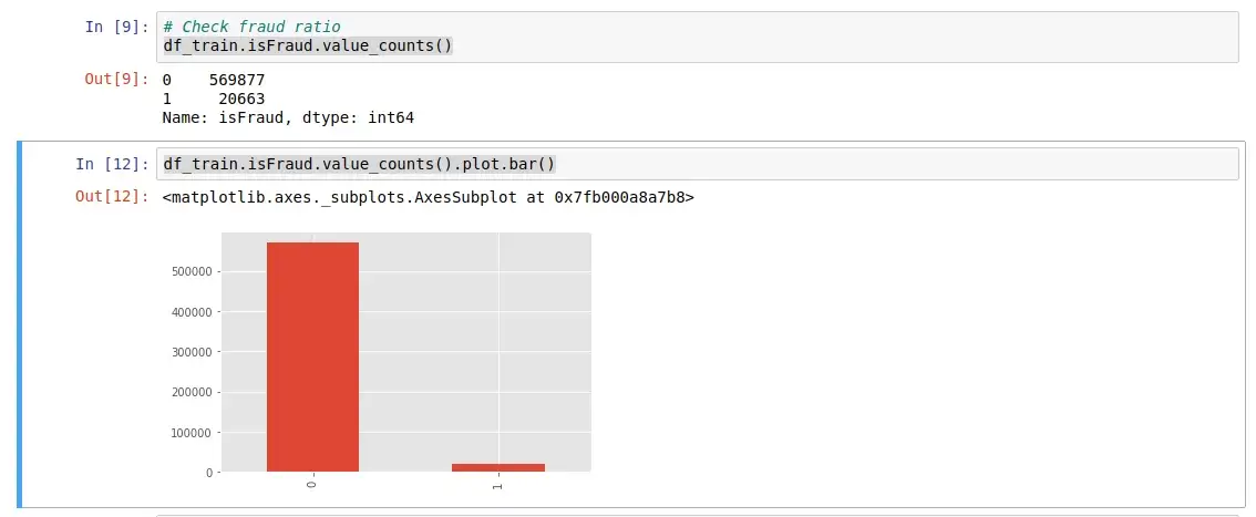
The dataset contains 20,633 frauds out of 590,540 records, that is hence highly imbalanced dataset.

df_train.isnull().sum()/len(df_train)*100    # missing ratio

This dataset also has high ratio of missing values, especially with features Addresses, Email, Device type, info and IDs.

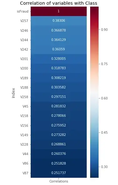
Let consider the correlation of different variables with the target variable

# Check the correlation of features with the target
import seaborn as sns
corr = df_train.corrwith(df_train.isFraud).reset_index()
corr.columns = ['Index', 'Correlations']
corr = corr.set_index('Index')
corr = corr[abs(corr.Correlations) > 0.25]
corr = corr.sort_values(by=['Correlations'], ascending = False)
plt.figure(figsize=(4,10))
fig = sns.heatmap(corr, annot=True, fmt = "g", cmap="RdBu_r")
plt.title("Correlation of variables with Class")
plt.show()

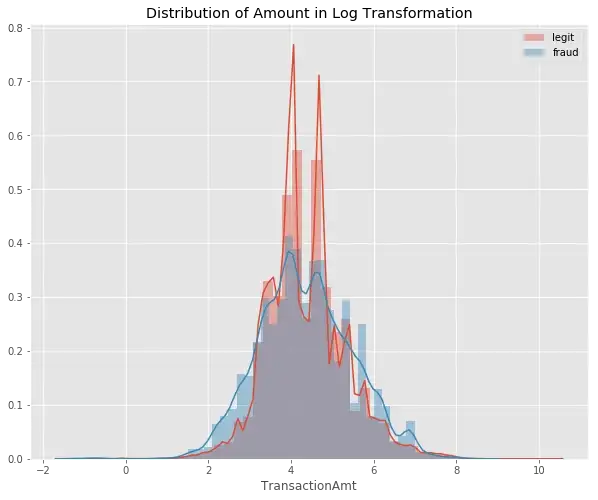
Distribution of Log Transaction Amount

#plot the amount feature
plt.figure(figsize=(10,8))
plt.title('Distribution of Amount in Log Transformation')
sns.distplot(np.log(df_train[df_train['isFraud']==0]['TransactionAmt']));
sns.distplot(np.log(df_train[df_train['isFraud']==1]['TransactionAmt']));
plt.legend(['legit','fraud'])
plt.show()

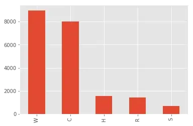
Frauds in IEEE-CIS dataset

We can further perform analysis on frauds of IEEE-CIS dataset. At first, let’s consider what types of product frauders performed:

df_fraud = df_train[df_train.isFraud == 1]
plt.ylabel('type')
df_fraud.ProductCD.value_counts().plot.bar()

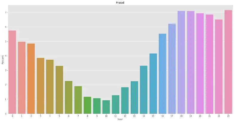
Let’s see the distribution of frauds based on time purchased (hour or day):

df_fraud['hour'] = (df_fraud['TransactionDT']//(3600))%24
df_test['hour'] = (df_test['TransactionDT']//(3600))%24
plt.figure(figsize=(20,10))
percentage = lambda i: len(i) / float(len(df_fraud['hour'])) * 100
ax = sns.barplot(x = df_fraud['hour'], y = df_fraud['hour'],  estimator = percentage)
ax.set(ylabel = "Percent")
plt.title('Fraud')

df_fraud['day'] = (df_fraud['TransactionDT']//(3600*24))%7
plt.figure(figsize=(15,10))
percentage = lambda i: len(i) / float(len(df_fraud['day'])) * 100
ax = sns.barplot(x = df_fraud['day'], y = df_fraud['day'],  estimator = percentage)
ax.set(ylabel = "Percent")
plt.title('Fraud')

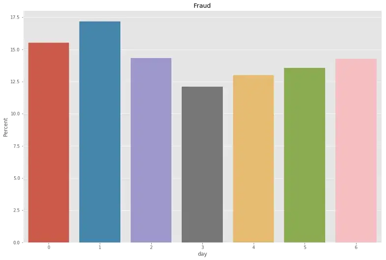
From hour-based, we can see that more frauds are performed from 4:00pm till 2:00am and less frauds performed in the daylight time. There is no significant different among days in terms of frauds.

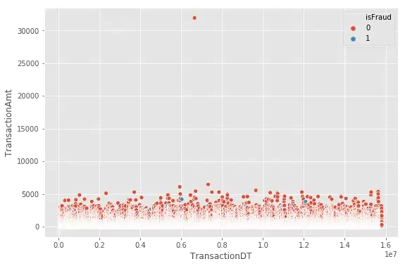
Now, let’s visualize frauds in the whole dataset

plt.figure(figsize=(9,6))
sns.scatterplot(x="TransactionDT",y="TransactionAmt",hue="isFraud", data=df_train)

Isolation Forest

Isolation Forest is a tree ensemble learning model, aims at detecting anomalies without profiling normal data points in advance. Isolation Forest is built on the basis of decision trees in which each tree divides the problem space into a set of partitions.

In Isolation Forest, the partitions are created by first randomly selecting a feature and then selecting a random split value between the minimum and maximum value of the selected feature. Basically, each isolation tree is created by firstly randomly sampling N instances from the training dataset. Then, at each node:

1. Randomly choose a feature to split upon.
2. Randomly choose a split value from a uniform distribution spanning from the minimum value to the maximum value of the feature chosen in Step 2.

These steps are repeated until all N instances from dataset are “isolated” in leaf nodes of the isolation tree.

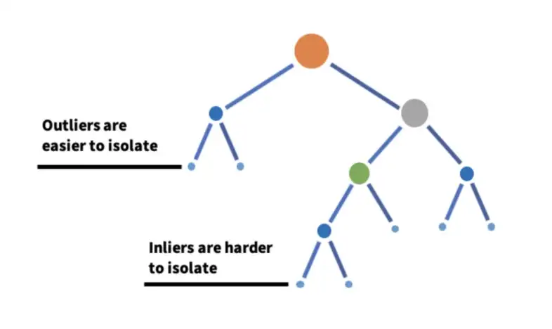
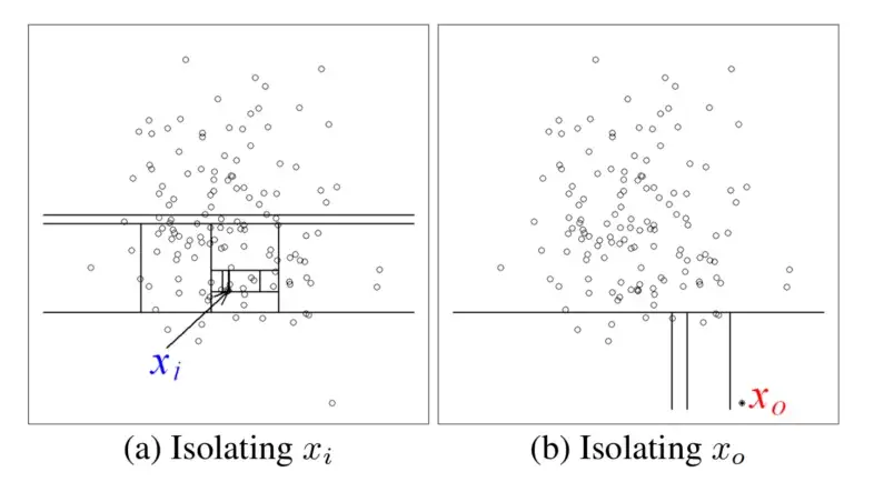
Basically, anomalies are less frequent than normal data and are different from them in terms of values. They lie further away from the normal data in the feature space. Thus, they could be identified closer to the root of the tree by using such a random partitioning.

Isolation Forest was implemented in the sklearn python package. It has the following hyperparameters:

• n_estimators: int, optional (default=100). The number of base estimators in the ensemble.
• max_samples: int or float, optional (default=”auto”). The number of samples to draw from X to train each base estimator.
• contamination: ‘auto’ or float, optional (default=’auto’). The amount of contamination of the data set, i.e. the proportion of outliers in the data set. Used when fitting to define the threshold on the scores of the samples.
• max_features: int or float, optional (default=1.0). The number of features to draw from X to train each base estimator.
• bootstrap: bool, optional (default=False). If True, individual trees are fit on random subsets of the training data sampled with replacement. If False, sampling without replacement is performed.

from sklearn.ensemble import IsolationForest
#split dataset
#fit model
clf = IsolationForest(max_samples = 256)
clf.fit()