Understanding KZG Polynomial Commitment Scheme

Cryptographic Commitments

Cryptographic commitment schemes play an important role in cryptography world. They could be a building block in various protocols, such as zero-knowledge proofs, secure multi-party computation, verifiable secret sharing, etc. The commitment schemes ensure fairness, security, and privacy in their applications.

A commitment scheme consists of two phases:

• Commit phase: the sender computes a commitment $com$ to the secret value $m$ that he chose, that is, $com = commit(m)$.
• Reveal phase: the sender reveals the secret value and the receiver verifies if it is corresponding to its commitment.

A commitment scheme MUST provide two security features:

• Binding: the sender could not show two valid values $m_1, m_2$ for a commitment $com$, that is, $com = commit(m_1)$, and $com = commit(m_2)$.
• Hiding: the commitment reveals nothing about the committed value.

The commitment schemes could be either non-functional or functional. The former can solely commit and hide a value until it is revealed later, it could not provide any further computation or interaction with the commitments. Otherwise, a functional commitment scheme provides additional properties beyond just hiding the value. It allows for some form of computation or interaction with the committed value while maintaining its security properties. This means that operations can be performed on the committed value without revealing it, or proofs about the committed value can be generated and verified without revealing it.

An example of non-functional commitment is the use of a hash function $H$ (e.g., SHA256) to commit a message $m$. We just have to hash $m$ with some randomness $r$, that is, $com = H(m, r)$, and to verify we just have to rehash the given message $m$ and the randomness $r$, then compare if the output is equal to the commitment $com$. Although this commitment scheme hides and binds the message $m$, we could not do any computation on the commitment. Real-world applications need more features than that.

A functional commitment (or commit to a function) allows you to do something more. For example, the KZG polynomial commitment scheme we are going to study in this post allows you to commit a polynomial $p(X)$, and after that allows you to generate a proof proving that $p(u) = v$ for two public values $(u, v)$. Moreover, with its homomorphic property, we can further perform arithmetic operations (i.e., addition and multiplication) over the committed values without revealing the original values.

There are three main functional commitments:

• Polynomial commitments: commit to a polynomial $f(X) \in \mathbb{F}_p[X]$. This type of commitments leads to the Groth16 and Plonk zero-knowledge proof protocols.
• Vector commitments: commit to a vector $\vec{u} =$ $(u_1, u_2, …, u_d) \in$ $\mathbb{F}p^{d}[X]$, and open a cell $f{\vec{u}}(i) = u_i$. A typical example of this is committing to a Merkle tree. This leads to the zk-STARK protocol.
• Inner product commitments: also commit to a vector $\vec{u} =$ $(u_1, u_2, …, u_d) \in$ $\mathbb{F}p^{d}[X]$, but open an inner product $f{\vec{u}}(\vec{v}) = (\vec{u}, \vec{v})$. This leads to bulletproof protocol.

KZG Polynomial Commitment

Again, a trivial scheme to commit a polynomial $f(x) = a_0 + a_1 \cdot x + \cdots + a_d \cdot x^d$ is to use a suitable hash function, e.g., $com_p = H(a_0, a_1, \ldots, a_d, r)$, where $r$ is a random number sampling from $\mathbb{F}_p$. The proof of that commitment $com_p$ will be a tuple $(a_0, a_1, \ldots, a_d)$, and $r$. However, this trivial scheme does not provide the following features:

• short proof: the proof size is $O(d)$, that could be large if the degree $d$ is large.
• fast verification: again, when $d$ is a large number, a large proof size could require a significant time to hash.
• zero-knowledge: this is the most important feature that we could achieve a zk-SNARK protocol. Once open the commitment, the polynomial in trivial scheme is no longer secret.

The KZG polynomial commitment scheme can achieve all the above features. It is based on cryptographic pairings over ellitpic curves and requires a trusted setup phase. The entire protocol is shown in the below picture (source: https://crypto.stackexchange.com):

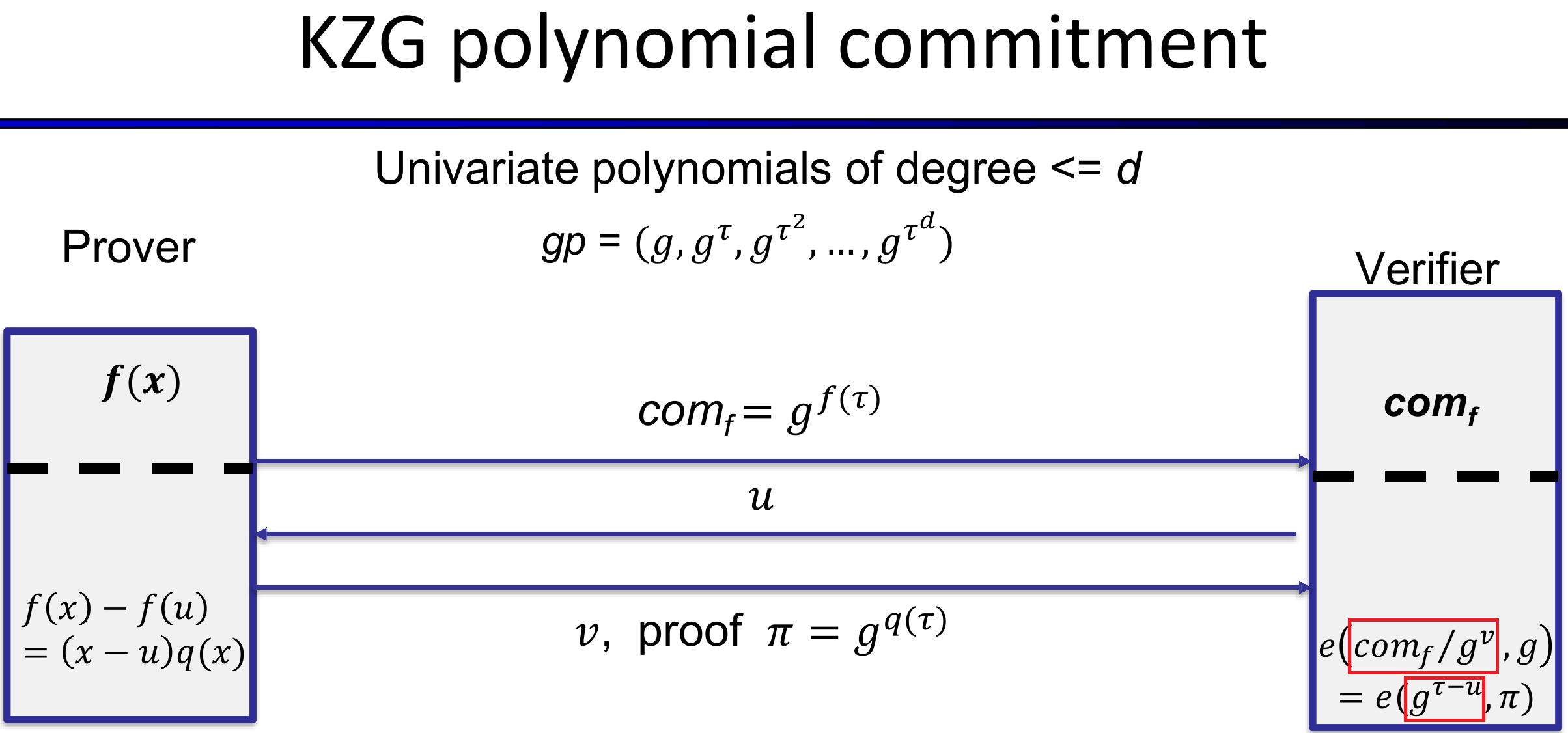
In more details, the KZG polynomial consists of the following steps:

• Step 1 (Trusted setup): A trusted server (or multiple participants joinly in a MPC protocol) generates a random secret value $\tau$, and computes the Structured Reference String (SRS), $gp = (H_0 = g, H_1 = g^{\tau}, H_2 = g^{\tau^2}, \ldots, H_d = g^{\tau^d})$. This global parameter SRS will be commonly used for any commitments.

from py_ecc.bn128 import G1, G2, multiply, add, neg, curve_order, Z1, pairing
import galois
import random

p = curve_order
GF = galois.GF(p)
tau = random.randint(1, p) 

powers_of_tau_G1 = [multiply(point, int(tau ** i)) for i in range(degree + 1)]   
tauG2 = multiply(G2, int(tau))

• Step 2 (Commit): To commit a polynomial $f(x) = \sum_{i = 0}^d a_i \cdot x^i$, the prover computes a commitment $com_f = g^{f(\tau)} = g^{\sum_{i = 0}^d a_i \cdot \tau^i} = \prod_{i = 0}^d (g^{\tau^i})^{a_i} = \prod_{i = 0}^d H_i^{a_i}$.

from functools import reduce
# Assume prover need to commit the polynomial f(X) = 5X^4 - 2X +3
fX = galois.Poly([5, 0, 0, - 2, 3], field = GF)
com_f = reduce(add, (multiply(point, int(coeff)) for point, coeff in zip(powers_of_tau_G1, fX.coeffs[::-1])), Z1)

• Step 3 (Verify): When a verifier wants to check the correctness of the committed polynomial $f(x)$, she chooses at random a value $u$, sends it to the prover who in his turn will compute a proof $\pi = g^{q(\tau)}$ where $q(X) = (f(x) - f(u))(x - u)$, and $g^{q(\tau)}$ is calculated in a similar way we did with $com_f$. The prover then sends the proof $\pi$ to the verifier, who in her turn will check the correctness of commitment $com_f$ by performing $2$ scalar multiplications, $2$ additions, and $2$ pairings over the pre-defined group of elliptic curve points.

# Verifier
u = random.randint(1, p) 
# Prover
v = fX(u)           
tX = galois.Poly([1, -u], field = GF)
qX = (fX - v) // tX
proof = reduce(add, (multiply(point, int(coeff)) for point, coeff in zip(powers_of_tau_G1[:d], qX.coeffs[::-1])), Z1)

# Verifier
uG2 = multiply(G2, int(u))
tau_minus_uG2 = add(tauG2, neg(uG2))
vG1 = multiply(G1, int(v))
com_f_minus_vG1 = add(com_f, neg(vG1))

if pairing(tau_minus_uG2, proof) == pairing(G2, com_f_minus_vG1):
  print("Proof for commitment is correct!")
else:
  print("Failed to test the proof!")

Unlike the trivial protocol showed above, the KZG commitment scheme holds the nice properties:

• short proof: the proof size is only one group element, i.e., a elliptic curve point over the underlying field $\mathbb{F}_p$ regardless the polynomial size.
• fast verification: fast with only $2$ scalar multiplications, $2$ additions, and $2$ pairings.
• zero-knowledge: the prover can generate a proof proving the correctness of the commitment without revealing any thing about the committed polynomial.

Now, let’s check if the KZG polynomial commitment scheme provides two security features: binding and hiding. It is obviously the scheme can hide the original value. Before showing the KZG poly commitment is binding, let’s recall the Schwartz-Zippel lemma:

Schwartz-Zippel Lemma: Let $f_1, f_2 \in \mathbb{F}^{(\le d)}_p[X]$ are two polynomials. If $f_1(r) = f_2(r)$ for some random value $r \in \mathbb{F}_p$, then $f_1 = f_2$ with high probability.

So, the Schwartz-Zippel lemma states that if two polynomials are evaluated at the same random value $r$, and return the same outputs, then one can be nearly certain that they are the same polynomial. This means that, once the prover committed a polynomial $f$, it would be infeasible for him to find another polynomial that produces the same commitment $com_f$. In other words, we say the polynomial $f$ binds to the commitment $com_f$.

Conclusions

KZG commitment scheme is foundational for some practical Zero-Knowledge Proof systems, including Groth16, Plonk, Halo, etc. Thus, understanding this underlying technique would help you to better understand the how ZKP systems are constructed. A full Python code of this post could be found in my GitHub repo. Hope you enjoy reading!