
Differential Privacy: An illustrated primer
Published:
Nowadays, many things you can do online, some can be named as browsing news, shopping, socializing, registering services, attending events and courses, visiting healthcare clinic, etc. Your life seems getting more and more convenient. However, the trade-off is that more and more your personal information is collected and used/shared over online platforms. You is becoming more visible on Internet, and hence getting higher risk to be a victime of online fraudulent activities.
So, we are concerned about our privacy with questions like: What is my data collected? How do they use my data? Are they going to share/sell my data to a 3rd party like what Facebook did to their users [1]? How my data is protected? etc. From service providers, they certainly want to maximize the benefits from data they collected. For example, sharing/selling to their partners, doing analysis to draw insights. From your side, you don’t want to be a part of the data that service providers are utilizing. For example, if Facebook is selling their users’ data, you hope that data does not contain yours. Whatever output drawn from the analysis won’t reveal any things about you. That is the core question Differential Privacy is trying to resolve.
To keep both sides achieving their goals, privacy-enhancing techniques (PET) could be used. They could be either cryptographic solutions such as zero-knowledge proofs, secure multi-party computation (SMPC), fully homomorphic encryption (FHE), etc., or non-cryptographic solutions such as data anonymization, synthetic data, differential privacy, etc. In which, Differential Privacy (DP) is a special tool that strikes a balance between your and service provider platforms’ goals.
In this post, I am going try to provide a (mostly) non-mathematical description of what differential privacy is and what makes it so promissing.
What is Differential Privacy ?
Differential Privacy (DP) is considered a promising approach to balance between protecting the individuals’ privacy and leveraging data for insightful analysis. The formal concept $\epsilon$-differential privacy was introduced in 2006 by Microsoft researchers Cynthia Dwork, Frank McSherry, Kobbi Nissim, and Adam Smith [2] as followed:
A randomized algorithm $\mathcal{A}$ with domain $\mathbb{N}^{\chi}$ is $(\epsilon, \delta)$-differentially private if for all subsets $\mathcal{S}$ of $\mathrm{im} \; \mathcal{A})$ and for all $D_1, D_2 \in \mathbb{N}^{\chi}$ such that $\parallel D_1 - D_2 \parallel _1 \, \le 1:$
\[\mathrm{Pr}[\mathcal{A}(D_1) \in \mathcal{S}] \le exp(\epsilon) \cdot \mathrm{Pr}[\mathcal{A}(D_2) \in \mathcal{S}],\]
where $\epsilon$ is a positive real number, $\mathrm{im}$ denotes the image of $\mathcal{A}$, and $\parallel D_1 - D_2 \parallel _1 \le 1$ means $D_1$ and $D_2$ differ on a single element (i.e., the data of one person). The probability is taken over the randomness used by the algorithm.
Basically, we need to add noise into queries/functions to private dataset. Dwork et al. formalized that amount of noise and also proposed a generalized mechanism for doing so. Prior to this work, Irit Dinur and Kobbi Nissim [3] proved that privacy could not be protected without adding some amount of noise. In addition, they showed that with a small number of random queries, a hacker can reveal the entire content of a private dataset.
In Dwork et al. formula above, $\epsilon$ means the privacy loss parameter. It determines how much noise that will be added to the computation. The smaller $\epsilon$ offers the better privacy, and otherwise, the bigger $\epsilon$ the more privacy lost. Of course, the ideal value is $\epsilon = 0$, however, at such a privacy level, the published data may not be accurate and hence not useful for further analysis. On the other hand, the value of $\epsilon$ should be not too big that will lead to leak private information. A recommendation given in [4] suggested that $\epsilon$ should be approximately between $0.001$ and $1$.
Interpret the formula
Probability of outcome S from dataset D_1
How similar the probability outcomes
A ‘real world’ example
Let consider a dataset of information of employees and their salaries in a company ABC as in the below table
| No. | Name | Salary |
|---|---|---|
| 1 | Alice | $90,000 |
| 2 | Bob | $125,000 |
| 3 | Charlie | $80,000 |
| 4 | Dragon | $95,000 |
| 5 | Eve | $110,000 |
| 6 | Floren | $70,000 |
| 7 | Geoffery | $65,000 |
| 8 | Huff | $100,000 |
| 9 | Kevin | $150,000 |
| … | … | … |
| 100 | Zayden | $130,000 |
In this example,
- $\mathbb{N}^{\chi}$ can be seen as the entire dataset of all one hundred (100) employees.
- $D_1$ and $D_2$ could be two datasets, which differ by only a single elemnet. For example $D_1$ is the set of first 8 employees and $D_2$ is the set of first 9 employees.
Now, the company ABC wants to publish the average of their employees. Assuming that a requester can send a query $\mathcal{Q}$ on an arbitrary number of employees of his choice. He sends two queries on $D_1$ and $D_2$ as above, that is $\mathcal{Q}(D_1)$ and $\mathcal{Q}(D_2)$. The returned results will be $91,875$ and $98,333$, respectively. Based on these two average numbers, the requester learnt about the salary of Kevin, which is $150,000$/year.
Now if we add some noise to the result of queries by applying a randomized algorithm $\mathcal{A}$ on two above datasets. This would return different results for different queries, even on the same dataset. For example, if $\mathcal{A}(D_1) = 95,000$ and $\mathcal{A}(D_1) = 96,000$, the attacker may just get very little information about Kevin’s salary. Even if the attacker is able to query multiple times on the two datasets above, the randomized algorithm $\mathcal{A}$ will return a new noised result for each query.
Let’s connect this example to formal definition. Assume that the expected avarage salary that the company ABC want to publish is $100,000$. The formula $\mathrm{Pr}[\mathcal{A}(D_1) = 100,000] \le exp(\epsilon) \cdot \mathrm{Pr}[\mathcal{A}(D_2) = 100,000]$ should be hold for a pre-defined value of $\epsilon$. Let’s say, the company provides a strong privacy for their employees, $\epsilon$ could be equal to $0.01$. The formula would be $\mathrm{Pr}[\mathcal{A}(D_1) = 100,000] \le 1.01 \cdot \mathrm{Pr}[\mathcal{A}(D_2) = 100,000]$, that is, the difference between two probabilities when querying $D_1$ and $D_2$ return to $100,000$ is about $1\%$, whether or not the data entry #10 included in the data requested. In other words, the chance the attacker discover Kevin’s salary increases at most by $1\%$.
The Laplace mechanism
The Laplace mechanism adds noise to the result of a query. The added value is sampled from a Laplace distibution (the figure below. Source: real-statistics.com).
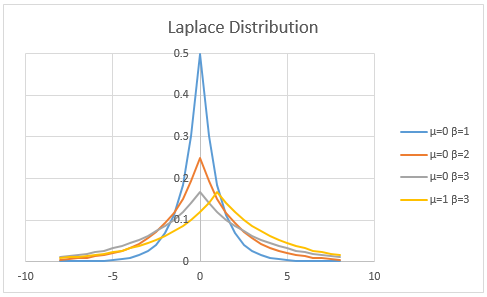
Formally, the probability density function of a variable that has a Laplace distribution is: \(L(x\mid \mu, \beta)={\frac {1}{2\beta}}\exp \left(-{\frac {|x-\mu |}{\beta}}\right),\,\!\) where $\mu$ is a location parameter, and $\beta$ a scale parameter that controlling the spread of the distribution. Like the normal distribution, this distribution is symmetric, converging to the location $\mu$. Compared to the normal distribution, Laplace distribution is more spread (i.e., having longer tails).
So, given a query $\mathcal{Q}$, the Laplace mechanism will return a result as:
\[\mathcal{A}(D) = \mathcal{Q}(D) + L(\mu, \beta)\]DP is quantifiable
Final notes: Differential Privacy is a quantifiable measure as with a mechanism and its parameter applied to a function (i.e., query), it is able to determine the privacy loss value $\epsilon$, which represents the privacy budget allocated to the algorithm. A smaller epsilon value implies a stronger privacy guarantee and a greater amount of noise added to the data, while a larger epsilon value implies a weaker privacy guarantee and a smaller amount of noise added to the data.
Additionally, differential privacy provides a mechanism for measuring the tradeoff between privacy and utility. Specifically, differential privacy provides a formal definition of the accuracy or quality of the output produced by a differentially private algorithm, which can be quantified using statistical measures such as mean squared error or absolute error.
In [2], Dwork et al. showed that by applying Laplace mechanism, the privacy loss parameter $\epsilon$ will be calculated as $\Delta\mathcal{Q}/\beta$, where $\Delta\mathcal{Q}$, so-called sensitivity, is a constant depending on the query $\mathcal{Q}$.
References
- Wikipedia, Facebook–Cambridge Analytica data scandal
- Cynthia Dwork, Frank McSherry, Kobbi Nissim, and Adam Smith, Calibrating noise to sensitivity in private data analysis. In Proceedings of the Third conference on Theory of Cryptography (TCC’06).
- Irit Dinur and Kobbi Nissim. 2003. Revealing information while preserving privacy. In Proceedings of the twenty-second ACM SIGMOD-SIGACT-SIGART symposium on Principles of database systems (PODS ‘03).
- Kobbi Nissim, Thomas Steinke, Alexandra Wood, Mark Bun, Marco Gaboardi, David R. O’Brien, and Salil Vadhan, Differential Privacy: A Primer for a Non-technical Audience